
Speeding Up SAC with Massively Parallel Simulation
Using SAC to meet and exceed the speed of tuned PPO on massively-parallel environments with simple implementation details and hyperparameter tuning.

Code: https://github.com/haosulab/ManiSkill/tree/fast_sac/examples/baselines/sac
WandB: https://wandb.ai/arth-shukla/ManiSkill-Fast-SAC
In recent years, GPU-parallelized simulation has made it possible to simulate thousands of trajectories in mere seconds. Moreover, Proximal Policy Optimization (PPO) has become the go-to RL algorithm for researchers and practitioners alike due to its ability to leverage the high throughput of massively parallel simulation.
However, on-policy RL algorithms like PPO have notable limitations in data efficiency and data sources. While these limitations are addressed by off-policy RL methods such as Soft Actor-Critic (SAC), off-policy methods are not typically tuned to take advantage of massively parallel simulation.
This goal of this post is to show that SAC without compile/CudaGraphs can be straightforwardly tuned to match and even beat tuned PPO with CudaGraphs baselines in wall-time speed on GPU-accelerated manipulation tasks from ManiSkill.
Why Off-Policy RL?
The shortcomings of on-policy RL
On-policy RL requires unbiased gradient estimates of the current policy, meaning we must update on data sampled from the current policy (or near-current in the case of PPO, which uses tricks like clipping, KL early stop, etc to allow for multiple updates on the same batch without exiting the trust region). Hence, if we collect a fresh batch of data from our current policy, after only a few updates this data will no longer match our current policy’s behavior, and we must throw it all away.
While the stale data problem is minimized by the high throughput of GPU-parallelized simulation, the true drawback here is that PPO cannot directly train on data from other sources (demonstrations, other policies, etc), which greatly limits its flexibility.
Off-policy RL is flexible
On the other hand, off-policy RL first trains value functions to estimate the expected return (usually a state-action value function, or Q-function). Then, for continuous action spaces, the policy is optimized to maximize Q-values from our learned Q-functions. Since the Q-functions can be updated using samples from any source, off-policy RL methods are compatible with demonstration data (teleoperated, machine-generated, etc), data sampled across policies, and data from prior experiments (e.g. QDagger, Replay Across Experiments). This enables creative, unique frameworks in Hierarchical RL (e.g. PEAR), learning from demonstrations (e.g. RFCL), and more.
Then why is PPO still more popular?
Since off-policy RL methods can update on the same data multiple times, they are typically much more sample-efficient than on-policy methods. As a result, works like REDQ and RLPD focus on tricks to make SAC (and its variants) much more sample-efficient rather than wall-time efficient.
One prior work in fast Q-learning is Parallelized Q-Learning (PQL), a distributed RL framework based on DDPG with mixed exploration noise that achieves SOTA wall-clock efficiency on IsaacGymEnvs. However, PQL has not yet seen widespread adoption at the level of PPO. While the reason is not fully clear, this may be partially due to the added complexity of its distributed framework compared to standard, sequential online RL.
Similar to this post, PQL also provides a SAC baseline which uses many environments, large batch size, and low UTD. However, this SAC baseline generally performs worse than PPO in their experiments, and it does not include other standard tricks like layer norm, varying Q/policy/Q-target ratios, etc.
Another recent work is Value-Based Deep RL Scales Predictably, which computes scaling laws for data and compute based on the update-to-data ratio (UTD). Slightly different from this paper (which updates the actor once per environment step and critic based on UTD), we find that tuning Q/policy/Q-target update ratios (e.g. 1-5 policy updates every critic update) results in faster wall-time on our tested tasks.
Hence, this post aims to demonstrate that a fairly standard SAC implementation with simple tricks can meet and exceed the wall-time performance of tuned PPO+CudaGraphs baselines on massively parallel environments from ManiSkill with simple implementation tricks and hyperparameter tuning.
Experimental Setup
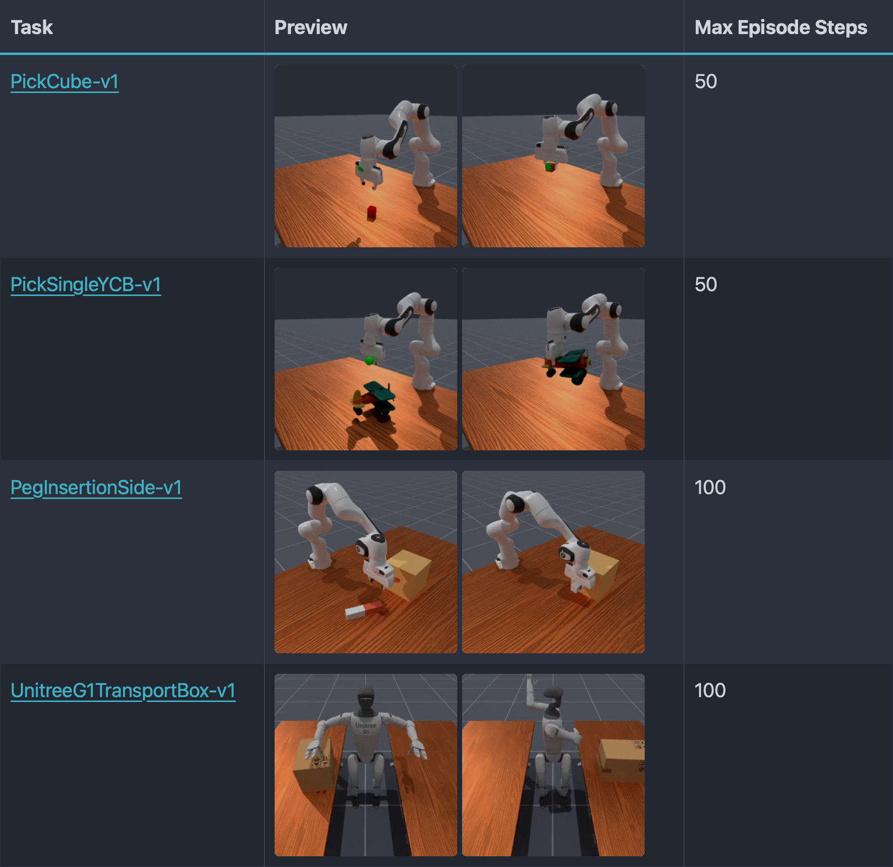
Simulator/Task Suite: ManiSkill
We test on four tasks from ManiSkill, a GPU-parallelized simulation framework targeted at robotic manipulation tasks. ManiSkill provides extensive, well-tuned baselines and out-of-the-box support for normalized dense rewards and action spaces.
SAC Implementation Details
Implementation
The provided implementation uses bog-standard PyTorch without torch.compile or CudaGraphs. The SAC implementation is fairly standard, using common tricks:
LayerNorm: Avoids critic divergence (per RLPD) with minimal extra computation.
Varying Q/Policy/Q-Target Update Ratios: While SAC will typically learn well-enough under standard ratios, tuning these can yield large speed benefits (in a sense, similar to tuning num epochs/num minibatches in PPO).
(Optional) Running Mean/STD Observation Normalization: This is used only in our PickCube tests, where we share SAC results with and without observation normalization. For the remaining tasks, this is disabled.
(Supported, unused) Q Ensemble: While critic ensembles can greatly improve sample efficiency, they are not as useful with high environment throughput and low update-to-data (UTD) ratio.
Tuning for Env Parallelism
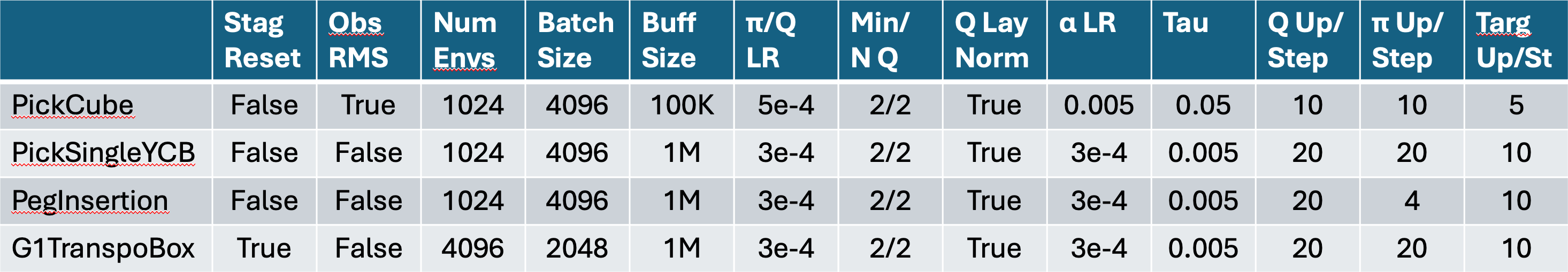
A full list of hyperparameters per environment is available in Appendix A.
Very low UTD and large batch size: As most SAC implementations are tuned for sample efficiency, they often tune UTD∈[0.2, 20]. However, with >1000 parallel environments, even UTD=0.2 requires hundreds of updates per environment step. Here, we use a very low UTD≤0.02, as we can collect large amounts of data for cheap. We also use larger batch sizes (2048-4096) to stabilize training.
Intuitively, a large number of environments enables faster data collection and higher data diversity, large batch sizes stabilize training, and very low UTD reduces time spent updating (which is fine, as we are able to sample more data very quickly regardless).
Q/Policy/Q-Target Update Ratios: We use a standard 10-20 Q-function updates per environment step. We additionally update the policy every 1-5 Q-function updates, and the Q-target every 1-2 Q-function updates. For notation, we say 20/20/10 update ratios means 20 Q updates, 20 policy updates, and 10 Q-target updates per environment step.
Final sweep params:
Num envs ∈ {1024, 2048, 4096} (default to 1024)
Batch size ∈ {1024, 2048, 4096, 8192} (default to 4096)
Update ratios: 20/20/10, 20/5/10, 10/10/5, etc (default to 20/20/10)
For simplicity, we keep learning rate, buffer size, etc the same for PickSingleYCB, PegInsertionSide, and UnitreeG1TransportBox. We make an exception for PickCube, the easiest task in our suite. Because PickCube is fairly easy to solve, we can use higher learning rate, more aggressive Q-target polyak averaging, smaller buffer size, etc, without worrying about training instability.
Staggered Reset
We also test staggered resets, where we spread environment resets across steps rather than resetting every environment at once. For example, if we have 2000 environments, truncate episodes at 100 steps, and ignore termination signals, then we can split the parallel environments into 100 buckets of 20, resetting a different bucket each environment step.
This trick is used often with PPO in legged locomotion to stagger certain environment behaviors (e.g. pushing robot) across batches, yielding more stable updates. Moreover, manipulation tasks are inherently staged: as the policy improves during training, our goal is to use staggered resets to include samples across task stages every environment step, increasing data diversity.
However, staggering resets can slow down rollouts via more-frequent, small-batch resets. As a result, staggered resets only sometimes yield improved wall-time results (for both SAC and PPO) which we discuss further in Appendix B.
PPO Baselines
We use the tuned PPO + CudaGraphs baselines provided by ManiSkill. It is important to emphasize: while the PPO baselines use CudaGraphs to optimize speed, our SAC implementation currently uses no such optimizations. The provided SAC results can be made even faster with torch.compile/CudaGraphs support. We also test PPO with staggered resets for fair comparison.
Results
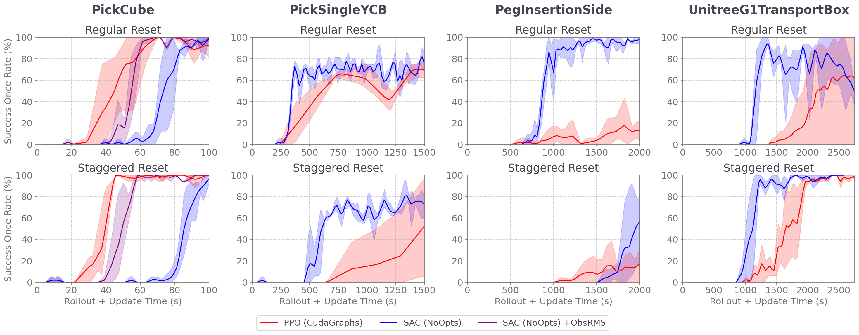
Metrics
We plot evaluation success once rate (i.e. % of episodes with at least one sample in success) over rollout+update time as training progress. We plot averages over 3 seeds with 95% CIs in the shaded regions.
Comparison
As seen above, SAC beats PPO+CudaGraphs wall-time in PickSingleYCB and PegInsertionSide with and without staggered resets. (Note that PickSingleYCB is partially observable even with state observations, so both methods level out at ~70% success once rate). For UnitreeTransportBox, SAC beats PPO with staggered resets; however, while SAC converges faster without staggered resets, it converges worse than PPO.
In PickCube, the easiest environment to solve, PPO decidedly beats SAC, solving 50% faster. Even when provided with running mean/std observation normalization, SAC (with or without staggered resets) is still slightly slower than PPO with staggered resets.
Conclusions, Weaknesses, and Future Work
We show that a well-tuned, fairly standard SAC with good implementation not only performs well wall-time on GPU-parallelized ManiSkill manipulation tasks, but also beats tuned PPO+CudaGraphs baselines on harder tasks. However, additional code optimizations and tricks are needed to help SAC reach the speed of PPO on easier tasks like PickCube.
Furthermore, enabling staggered reset should be chosen wisely. As discussed further in Appendix B, staggered resets can inflate rollout time if environment resetting is slow. So, staggered reset should only be enabled if environment resetting is fairly fast. Under this methodology, SAC consistently outperforms PPO+CudaGraphs wall-time on the harder environments we test.
One major weakness of these tests is we rely on normalized action spaces and rewards provided by ManiSkill. As noted by Anton Raffin in Getting SAC to Work on a Massive Parallel Simulator, many tasks purposefully allow for unbounded action spaces, e.g. with joint position control to allow the robot to output larger joint torques while still being compatible with standard, high-frequency PD controllers. Furthermore, many regularization terms necessary for sim2real (e.g. slippage, torque penalties, etc) can be difficult to scale 0-1 (e.g. with tanh), and would require additional tuning and trial-and-error.
Future work includes adding compile/CudaGraphs support for even faster training and implementing the same tricks/tuning with other off-policy methods.
Acknowledgement
Many thanks to Stone Tao, Nicklas Hansen, and Zhiao Huang for their feedback!
Appendix
A - Hyperparameters
B - Why does staggered reset sometimes yield slower wall-time training?
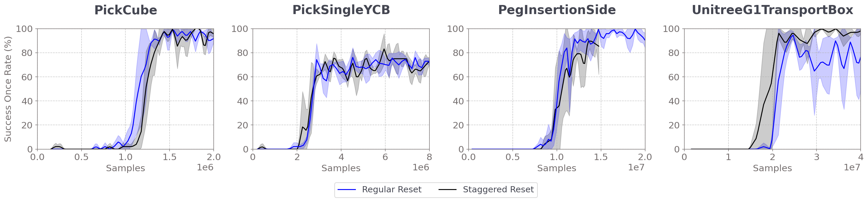
First, we observe that sample efficiency is comparable even in PickSingleYCB and PegInsertionSide, where training with staggered reset was notably slower wall-time than with regular reset.
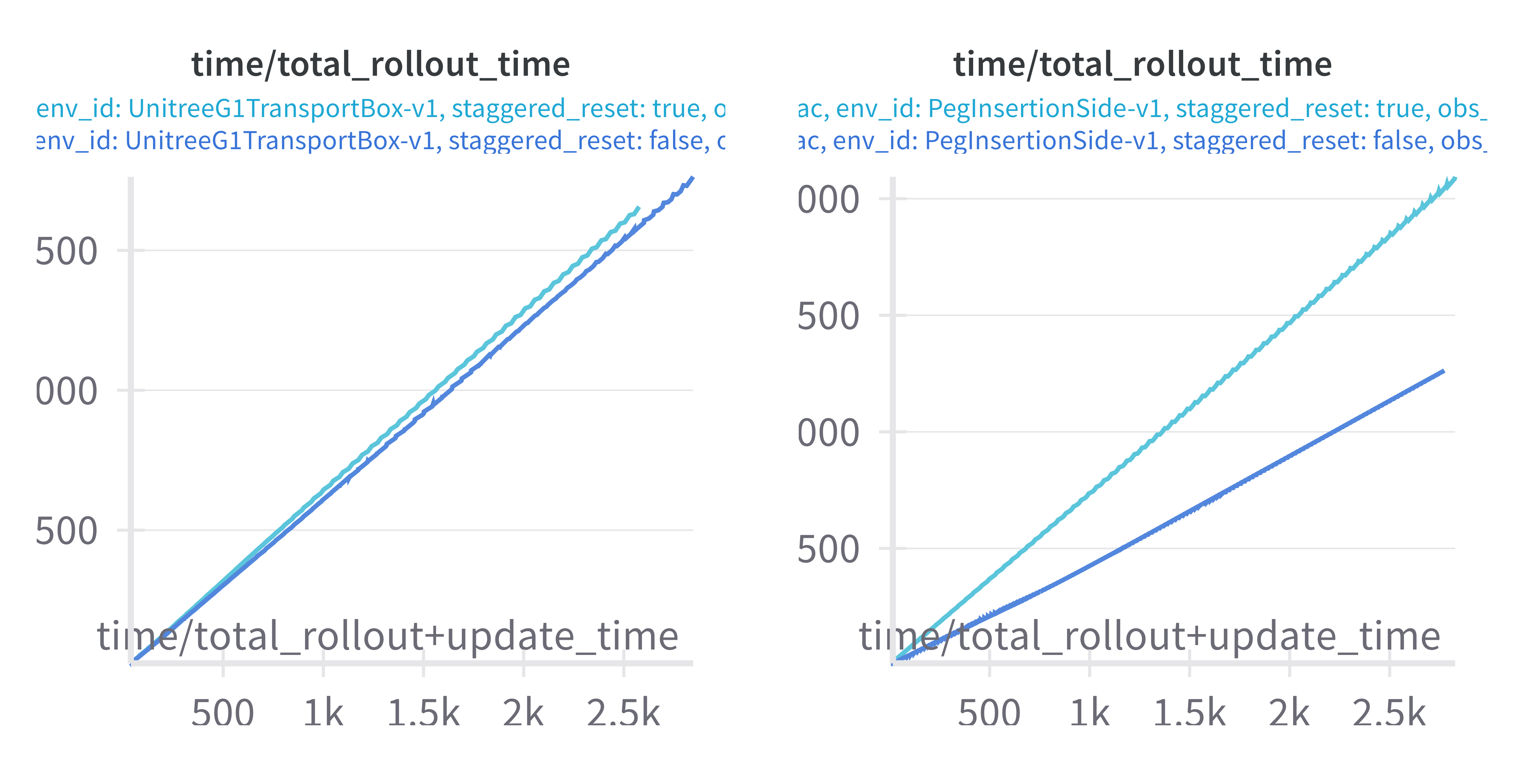
Furthermore, we see in UnitreeG1TransportBox that rollout time with and without staggered reset is comparable, but in PegInsertionSide rollouts are 40% slower with staggered reset. So, while staggered reset can improve convergence, if resetting an environment is slow, then the gains from staggered reset are lost to increased rollout time.
Hence, it is best to briefly test rollouts with and without staggered reset. If the time difference is not too great, then using staggered reset is recommended. However, if staggered reset notably slows down simulation, then initial experiments should disable this feature.
Citation
@article{shukla2025fastsac,
  title   = "Speeding Up SAC with Massively Parallel Simulation",
  author  = "Shukla, Arth",
  journal = "https://arthshukla.substack.com",
  year    = "2025",
  month   = "Mar",
  url     = "https://arthshukla.substack.com/p/speeding-up-sac-with-massively-parallel"
}